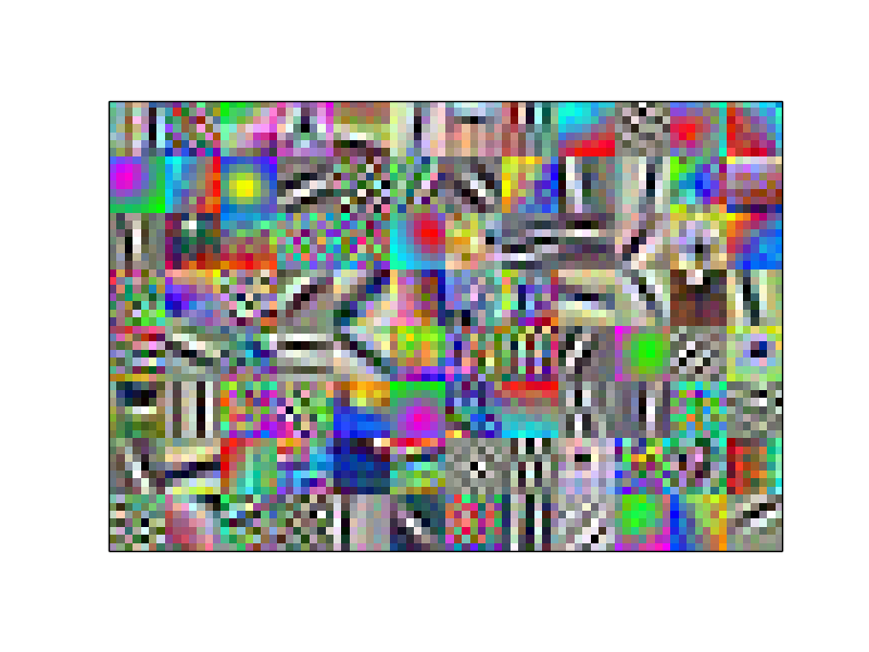
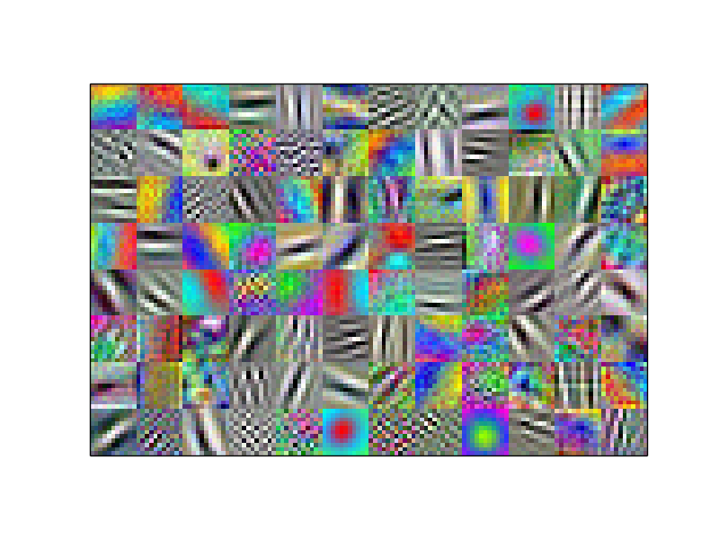
Visualization of first layer filters¶

The first layers of convolutional neural networks often have very “human interpretable” values, as seen in these example plots. Visually, these filters are similar to other filters used in computer vision, such as Gabor filters.

Python source code: plot_overfeat_layer1_filters.py

print(__doc__)
import numpy as np
import matplotlib.pyplot as plt
from sklearn_theano.feature_extraction import fetch_overfeat_weights_and_biases


def make_visual(layer_weights):
    max_scale = layer_weights.max(axis=-1).max(axis=-1)[...,
                                                        np.newaxis, np.newaxis]
    min_scale = layer_weights.min(axis=-1).min(axis=-1)[...,
                                                        np.newaxis, np.newaxis]
    return (255 * (layer_weights - min_scale) /
            (max_scale - min_scale)).astype('uint8')


def make_mosaic(layer_weights):
    # Dirty hack (TM)
    lw_shape = layer_weights.shape
    lw = make_visual(layer_weights).reshape(8, 12, *lw_shape[1:])
    lw = lw.transpose(0, 3, 1, 4, 2)
    lw = lw.reshape(8 * lw_shape[-1], 12 * lw_shape[-2], lw_shape[1])
    return lw


def plot_filters(layer_weights, title=None, show=False):
    mosaic = make_mosaic(layer_weights)
    plt.imshow(mosaic, interpolation='nearest')
    ax = plt.gca()
    ax.xaxis.set_visible(False)
    ax.yaxis.set_visible(False)
    if title is not None:
        plt.title(title)
    if show:
        plt.show()

weights, biases = fetch_overfeat_weights_and_biases(large_network=True)
plot_filters(weights[0])
weights, biases = fetch_overfeat_weights_and_biases(large_network=False)
plt.figure()
plot_filters(weights[0])
plt.show()

Total running time of the example: 0.40 seconds ( 0 minutes 0.40 seconds)